Where and Why "Eval" Goes Wrong

You run your evaluation on 100 test cases and get 82%. How confident should you be in that number? Do you know? Do you think the people reporting on the eval know? Do you think the team listening to the presentation know?

My experience is that even among attendees of scientific conferences, most people don't know. I guarantee that the average listener of reports on AI eval in companies does not know.

The answer, by the way, is nuanced and somewhat depends on assumptions and on the "mean" accuracy, but a ballpark estimate is that with 100 data points at a mean accuracy of 82%, the 95% confidence interval is roughly 16 points wide. The true accuracy could plausibly be anywhere from 74% to 90%.

And this is enough to flip your decisions.

Just to be clear: the interval is ONLY 16 points wide if you make a lot of optimistic and likely unrealistic assumptions, that we can sum up as "the only source of uncertainty is the sample size". That's never the case.

This begins to show that the report may not just be meaningless, but also misleading. And if as listener we do not ask questions, we are contributing to a culture that fosters random iterations in search for good solutions.

---

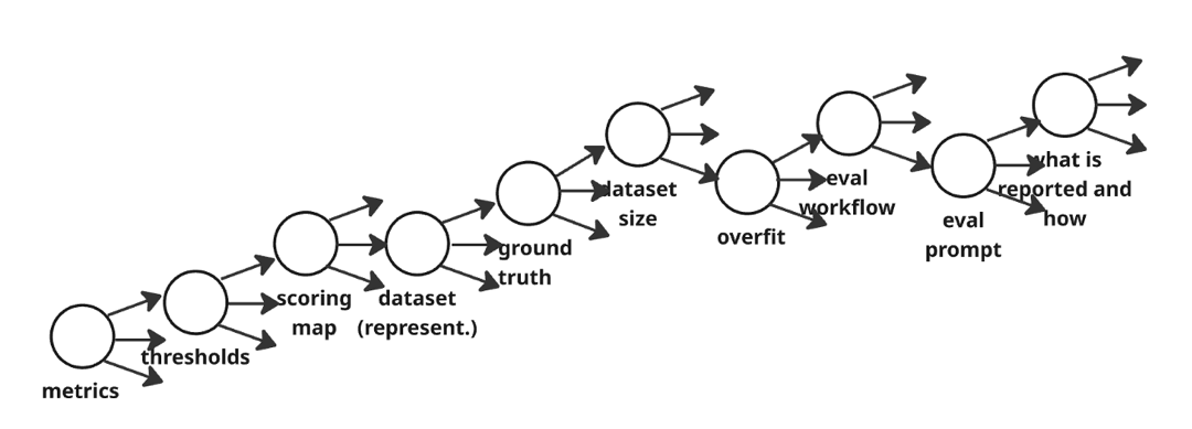
In Software 3.0, improvement is usually not a single leap, but a search process. You try a prompt tweak. You change the retrieval strategy. You reorder steps in the pipeline. You swap the judge prompt. You run the same evaluation suite again. Repeat.

This is a healthy engineering loop. But it changes what an evaluation score means. The moment we run many variants and report (or remember) the best-looking number, we have quietly introduced a statistical phenomenon that is both simple and surprisingly strong: multiple hypothesis testing.

Here, a "hypothesis" is not a formal paper claim. It is any variant we tried: a prompt version, a pipeline branch, a scoring rule, a filtering threshold, or even a different way to aggregate sub-metrics. Testing many hypotheses is not the problem. The problem is that selection ("pick the winner") converts random noise into systematic optimism.

The Dice Analogy

If you roll one fair die, the expected value is 3.5. If you roll 20 fair dice and keep the highest, the expected value is much higher—even though nothing about the dice improved. In evaluation, the "dice" are the random components of measurement: finite sample size, ambiguous ground truth, judge variability, and the many small implementation choices that leak into scores. The best score among many tries is expected to be "lucky".

The Best-of-K Effect

Let the observed score for variant i be a noisy estimate of its underlying performance:

observed_score_i = true_score_i + noise_i

Assume the noise terms are centered (the evaluation is not systematically biased for any single run), with standard deviation σ. If we run K variants and select the highest observed score:

selected_score = true_score + max(noise_1, ..., noise_K)

Even though each noise_i has mean 0, the maximum does not. The expected max is positive, so the selected score is systematically optimistic. This is the "winner's bonus".

Expected "winner's bonus" from selecting the best of K tries:

K variants tried	E[max noise]/σ	If σ = 4 points, expected bonus
1	0.000	+0.0 points
2	0.564	+2.3 points
5	1.163	+4.7 points
10	1.539	+6.2 points
20	1.867	+7.5 points
50	2.249	+9.0 points

By the time you have tried 10-20 variants, the expected winner's bonus is already around 1.5-1.9σ. That is not a rounding error if σ is several points.

From Test-Set Size to Best-of-K Inflation

To translate σ into something tangible, it helps to connect it to test-set size. For illustration, suppose the underlying accuracy is about 80%. The standard deviation of the measured accuracy from N cases is approximately sqrt(p(1-p)/N).

N test cases	σ (points)	Best-of-5 (+ points)	Best-of-10 (+ points)	Best-of-20 (+ points)
50	5.66	+6.6	+8.7	+10.6
100	4.00	+4.7	+6.2	+7.5
200	2.83	+3.3	+4.4	+5.3
500	1.79	+2.1	+2.8	+3.3
1000	1.26	+1.5	+1.9	+2.4

With N = 100 cases, the sampling-only σ is about 4 points, so best-of-20 inflation is about +7.5 points on average. And this is only sampling noise. In Software 3.0, the effective σ is often larger because the evaluation pipeline itself is stochastic or under-specified.

Why This Creates the Illusion of Progress

If none of the variants are truly better, how often will the best one still look meaningfully better?

Probability that best-of-K looks at least δ points better than truth (σ = 4 points):

Threshold δ (points)	Best-of-5	Best-of-10	Best-of-20
2	84.2%	97.5%	99.9%
4	57.8%	82.2%	96.8%
6	29.2%	49.9%	74.9%
8	10.9%	20.6%	36.9%

This explains a common experience in prompt engineering: you can "find" a 4-8 point improvement surprisingly easily when the test set is small and you iterate a lot—even if the underlying system has not improved.

The best-of-K inflation is real, but it compounds with two more fundamental problems:

Small sample sizes: If you're evaluating K variants on 100 examples, your confidence interval is already ~16 points wide before accounting for selection effects. Best-of-K adds optimism on top of already massive uncertainty.

Non-representative test data: Your test set is almost never IID with production. It's curated examples someone thought were representative, synthetic data that's "close enough," or historical data from a shifted distribution. This isn't noise—it's bias. Your evaluation could be perfectly precise and still systematically wrong because you're measuring on the wrong distribution.

If your 100-example test set doesn't reflect production, no statistical correction will save you.

A technical note: the standard best-of-K analysis assumes independent noise across variants. In practice, when variants share the same test set and judge, noise is partially correlated—which reduces but does not eliminate the inflation. The core insight holds: selection on noisy estimates produces optimistic results.

Three Context Questions

When you see a crisp green number, three context questions often unlock most of the uncertainty:

• How many variants were tried and compared on this same dataset?
• How noisy is one evaluation run (what is σ)?
• How wide was the search (were variants meaningfully different, or minor edits)?

Sadly, this is not a theoretical paranoia. It's real. You need to manage it.

---

Note: This section focuses specifically on bias introduced when developers tune prompts based on observing test cases—a distinct contribution to the gap between test and production performance.

The Mechanism: A Different Kind of Overfitting

Classical overfitting occurs when a model with too much capacity memorizes training data rather than learning generalizable patterns. What we observe in Gen AI evaluation is structurally different: the developer becomes the fitting agent, not the model.

Consider how prompt engineering typically works. A team builds an AI agent—say, a tool-calling agent for IT support. They create 50 or 100 test cases. They run the agent, observe failures, and iterate. They adjust the prompt, add in-context examples, tweak instructions. Test accuracy improves from 65% to 88%.

What happened during this process? The developer—consciously or not—learned the patterns in those specific test cases. Their intuitions about "what makes a good prompt" became shaped by those 50 examples. The in-context examples they added were chosen because they helped with the failures they observed.

This is not a failure of engineering discipline. This is normal, reasonable engineering behavior. The challenge is structural: this process changes the relationship between your test score and your production performance in ways that are difficult to detect.

When This is Good Engineering vs. Problematic Overfitting

If the test set is representative of production—if production users also frequently use the patterns in your test set—then tuning to observed patterns is good engineering.

The problem arises when the test set is not representative. If the test set over-represents certain patterns, under-represents others, or happens to contain spurious correlations, then each "improvement" potentially increases the gap between test and production performance.

The difficult part: these two scenarios look identical from the developer's perspective. The same test-set improvement—say, from 70% to 88%—could represent:

• Legitimate improvement that will fully transfer to production
• Partial improvement (perhaps 10 points real, 8 points overfitting)
• Overfitting that will not transfer to production

The test score alone cannot distinguish between these cases. Only held-out data or production results can reveal which occurred.

Example A: Lexical Overfitting

A team builds a password-reset agent. Their golden dataset of 100 test cases was curated by a QA team who wrote clear, well-formed queries like "I need to reset my password" and "Password reset request for SAP."

Production users don't write like QA teams: "cant log in keeps saying wrong password tried 3 times now HELP" or "locked out again ffs".

Phrasing Type	Test Set	Production
Clean phrasing	100%	35%
Messy phrasing	0%	65%

The agent achieves 94% accuracy on clean phrasing but only 71% on messy phrasing.

Metric	Value
Test Accuracy	94.0%
Production Accuracy	(0.35 × 94%) + (0.65 × 71%) = 79.1%
Bias (Test − Production)	14.9 percentage points

Example B: Distribution Mismatch in Tool Selection

An IT support agent can invoke five tools. Test cases are easy to write for some tools (Password Reset) but complex for others (Network Diagnostics).

Tool	Test Set Distribution	Production Distribution
Password Reset	31%	15%
KB Search	28%	20%
Ticket Creator	22%	15%
Network Diagnostics	12%	35%
Escalation	6%	15%

The agent has higher accuracy on over-represented tools (93% for Password Reset) and lower accuracy on under-represented tools (72% for Network Diagnostics).

Metric	Value
Test Accuracy	86.5%
Production Accuracy	78.6%
Bias	7.9 percentage points

Example C: Complexity Mismatch

Test cases were written by humans creating "good examples"—clean, single-intent, unambiguous queries. Production queries are messier: multi-intent requests that blend multiple issues in one rambling message.

Metric	Value
Test Accuracy	91.0%
Production Accuracy	71.7%
Bias	19.3 percentage points

Example D: Spurious Correlation in Tool Selection

A team notices that their 20 KB Search test cases all begin with a question word. They add an instruction: "If the user query begins with 'what,' 'how,' 'why,' or 'when,' consider KB Search."

Test accuracy improves from 83% to 89%. But in production, the correlation doesn't hold—only 55% of KB Search queries start with question words.

Metric	Value
Test Accuracy	89.0%
Production Accuracy	73.1%
Bias	15.9 percentage points

Summary: The Compounding Effect

Overfitting Type	Mechanism	Bias Introduced
Lexical overfitting	Test cases use phrasing that differs from production	14.9 points
Distribution mismatch	Some tools/intents over-represented in test set	7.9 points
Complexity mismatch	Test cases are cleaner than production queries	19.3 points
Spurious correlation	Pattern in test set doesn't hold in production	15.9 points

When multiple overfitting mechanisms operate together, their effects partially overlap but also partially compound. A test accuracy of 88% might translate to production accuracy anywhere from 60-78%.

---

So far we have discussed uncertainty arising from limited measurement and selection effects. We now turn to a different class of problems: errors introduced by how we encode quality itself.

Even when we have collected our data, run our evaluations, and obtained raw results from our LLM-as-judge or human raters, we still have to map those results to scores—and this mapping is far more arbitrary than most teams realize.

Suppose we use a prompt that judges "completeness" on a qualitative 1-3 scale:
- 1 = incomplete
- 2 = partially complete
- 3 = fully complete

We convert it to a percentage using a simple linear mapping. The result: 84% Completeness. Green box.

That linear mapping encodes an assumption—that the difference between a 1 and a 2 is the same as the difference between a 2 and a 3. Is that true?

Three Systems, Same Score, Radically Different Behavior

System	Count of 3s	Count of 2s	Count of 1s	Characterization
A	4	4	2	Mixed performance, some excellence
B	2	8	0	Consistent, no failures
C	6	0	4	Bimodal: great or terrible

Under the linear mapping, all three systems score exactly the same: 2.2 average, or 60%.

But these systems are radically different. Which would you rather deploy?

Five Reasonable Mappings, Five Different Winners

Mapping	Rationale	Score Values	Results	Winner
Linear	Equal intervals	1→0, 2→50, 3→100	A=60, B=60, C=60	TIE
Top-Heavy	"2 is barely acceptable"	1→0, 2→30, 3→100	A=52, B=44, C=60	C
Mid-Heavy	"2 is already quite good"	1→0, 2→70, 3→100	A=68, B=76, C=60	B
Quadratic	Capability grows with squared effort	1→0, 2→44, 3→100	A=58, B=56, C=60	C
Exponential	Each level represents exponentially more	1→0, 2→25, 3→100	A=50, B=40, C=60	C

Same raw data. Five different answers to "which system is best."

And note: every one of these mappings is reasonable. The choice between them is a value judgment about what matters—but it's a value judgment that is almost never made explicitly.

---

Most evaluation pipelines for Software 3.0 quietly assume something that feels 'Software 1.0-ish':
- There is a correct answer (ground truth), or
- There is a stable judge (human or LLM) who can reliably say whether the output is 'good,' 'accurate,' 'complete,' etc.

In gen AI products, both assumptions often fail—not because teams are sloppy, but because the object being measured is different.

Separating Three Phenomena

• Noisy ground truth: the labels/reference answers are imperfect
• Noisy judge: the rater (human or LLM) is inconsistent or error-prone
• Subjectivity: there may not be a single intended criterion; different users legitimately disagree

What Judge Noise Does to Reported Scores

If the true acceptance rate is T, but the judge has:
- α = probability of false positive (calling a bad output "good")
- β = probability of false negative (calling a good output "bad")

Then: Reported = α × (1 - T) + (1 - β) × T

This creates compression: all true scores get pulled toward a middle range. With α = 0.10 and β = 0.15:

True Pass Rate	Reported
50%	47.5%
70%	62.5%
80%	70.0%
90%	77.5%

A system that truly improved from 70% to 90% (20 points) would only appear to improve from 62.5% to 77.5% (15 points). The ruler got compressed. Progress looks smaller than it is.

Subjectivity: User Perception is a Distribution

For many gen AI features, the quality of an output is not a single value; it is a distribution over user judgments. Even if you could sample from your target population, different users will judge differently.

How much user-perceived quality varies depending on sample size:

True approval p	# users m	SE of average rating	Approx 95% half-width
80%	5	17.9 pts	±35.1 pts
80%	20	8.9 pts	±17.5 pts
80%	100	4.0 pts	±7.8 pts

Even when true approval is high, a small panel can easily look negative:

True approval p	Panel size m	P(panel majority dislikes)
80%	3	10.4%
80%	5	5.8%

Even if 80% of real users would approve, a 5-person panel will still end up majority-negative about 1 time out of 17—without anyone being irrational.

---

This section focuses on a specific and surprisingly large source of variability: small variations in the LLM judge prompt. Even with a deterministic judge (temperature 0), changing a few words in the rubric can move headline metrics by many points—sometimes enough to flip decisions or reverse model rankings.

Why This is Not "Just Variance"

When you vary the judge prompt, you are often not introducing randomness around a fixed ruler—you are changing the ruler. Judge prompts set the rubric, strictness, and attention.

So judge-prompt variation can show up as both:
- Between-prompt variability: different reasonable judge prompts give different scores on the same outputs
- Measurement drift: the reported metric moves because the measurement instrument moved, not because the system improved

The Key Reason Small Edits Can Cause Big Swings

• Borderline mass: many cases sit near pass/fail or near a rubric boundary
• Threshold shifts: the prompt changes how borderline cases are resolved
• Construct shifts: the prompt changes what "quality" means

If N = 100 and the score changes by 20 points, that means 20 of the 100 items changed verdict purely due to the judge prompt.

Examples of "Small" Judge-Prompt Edits That Are Not Small

1) Strictness language (threshold shift)
- "Be strict."
- "Penalize even minor errors."
- "If any factual error exists, the score must be ≤ 2."

2) Construct shift (what quality even means)
- "Focus primarily on factual accuracy" vs "Focus primarily on completeness."
- "Citations required" vs "Citations optional."

3) Rubric structure and ordering (salience effects)
- Same rubric, different order (factuality first vs style first)
- Same rubric, different emphasis ("must" vs "should")

Rank Reversal: Judge Prompts Can Flip Which System is "Better"

Two judge prompts with different emphases can produce opposite rankings:

Under Prompt 1 (factuality-first): Agent A = 3.7, Agent B = 3.3 → A wins

Under Prompt 2 (completeness-first): Agent A = 3.3, Agent B = 3.7 → B wins

What Borderline Mass Implies

Borderline fraction b	If 20% of borderlines flip	If 60% flip	If 80% flip
10%	2 points	6 points	8 points
20%	4 points	12 points	16 points
30%	6 points	18 points	24 points

This explains why 20-30 point swings are plausible even with deterministic judging: if a substantial fraction of your evaluation set is borderline and the judge prompt moves the boundary, the metric will move accordingly.

---